Simple example

This pages uses a simple experiment to illustrate some of the basic features of Phileas. It shows how to measure the values of a field at different spatial positions.

Experimental setup and drivers

This experiment is based on two instruments:

• a probe is used to measure the amplitude of the electric field. It is connected to an oscilloscope.

• A motorized stage is used to position the probe.

We want to plot different field maps, so for this we need to automate the positioning of the probe and the measurement of the field. Two drivers are used, allowing to control

• the maximum amplitude of the oscilloscope. It must be high enough to avoid saturation, but low enough to prevent quantization noise. Different amplitudes are tried to solve this issue.

• The motorized stage has thgrees of freedom, denoted \(X\), \(Y\) and \(Z\), which also computer-controlled.

This example uses simulated instruments, availabe in the phileas.mock_instruments module. They can be used as follows:

motors = mock_instruments.Motors()
probe = mock_instruments.ElectricFieldProbe(motors)
oscilloscope = mock_instruments.Oscilloscope(probe)
oscilloscope.amplitude = 1

print(f"Field value with {motors}: {oscilloscope.get_measurement()}")
motors.set_position(x=1, y=1.5)
print(f"Field value with {motors}: {oscilloscope.get_measurement()}")

INFO:phileas.phileas.mock_instruments:[Motors] Connection initiated.
INFO:phileas.phileas.mock_instruments:[Oscilloscope] Connection initiated.
Field value with Motors(x=0.0, y=0.0, id='mock-motors-driver:1'): 0.5
Field value with Motors(x=1, y=1.5, id='mock-motors-driver:1'): 0.0234375

probe.get_amplitude()

np.float64(0.024688715247306627)

If we break this down,

1. the drivers are instanciated,

2. the instruments are configured,

3. and finally, measurements are gathered.

We will now see how to use Phileas to automate these measurements for more positions.

Describing the experimental bench

The first step to drive the instruments is to describe what what instruments are available on the bench, and how to connect to them. This gives Phileas all the information required to instanciate the drivers. This is done by the bench configuration file, which is a simple YAML file. In our case, as the instruments are simulated, we can define it like this:

bench = """
simulated-motors:
    loader: phileas-mock_motors-phileas

simulated-oscilloscope:
    loader: phileas-mock_oscilloscope-phileas
    probe: electric-field-probe
    motors: simulated-motors
"""

This bench configuration states that two instruments, simulated-motors and simulated-oscilloscope are available. Then, it tells the simulated oscilloscope what probe is used, and how it is driven. Notice the loader attribute : it is a special field, which is required by Phileas for instantiating the drivers. It is explained in the following section.

See also

Bench configuration file further describes the syntax of this file.

Warning

Here, the content of the bench configuration file is stored in a Python str, as it integrates easily with notebooks. Usually, it is preferred to store it in a file, conventionally called bench.yaml.

Describing the instrument parameters

The instruments available on the bench can now be configured. This is the purpose of the experiment configuration file. It is also a YAML file, which describes

• what instruments are required by the experiment,

• how to configure them,

• and is usually used to document the experiment itself, working as a lab notebook.

Let us define it as

experiment = """
description: Measure the electric field for a single probe position.

motors:
    interface: 2d-motors
    x: 1
    y: 1.5

oscilloscope:
    interface: oscilloscope
    amplitude: 1
"""

It contains two entries motors and oscilloscope, which are identified as instrument entries by their interface key. It is a requirement, which states that instrument motors must be a 3d-motors. Phileas uses this internally to match the required instrument with the available ones. Besides the interface reserved keyword, each instrument entry describe its required configuration.

Finally, this file can also contain arbitrary data, which is convenient to document the experimental process. Here, the description entry simply states the purpose of the experiment, but it could be much more detailed.

See also

Experiment configuration file further describes the syntax of this file.

Warning

Here, the content of the experiment configuration file is stored in a Python str, as it integrates easily with notebooks. Usually, it is preferred to store it in a file, conventionally called experiment.yaml.

Letting Phileas handle instruments with loaders

The bench configuration file describes the available instruments of a bench, whereas the experiment configuration file requires some of them. Internally, Phileas relies on loaders to match the requirements to the available instruments.

A loader is a simple Python class, which

• is identified by a name, which is used in the bench configuration file. In this example, loaders phileas-mock_motors-phileas and phileas-mock_oscilloscope-phileas are used.

• Additionally, it has can support multiple interfaces, which are requested by the experiment configuration file. In this example, interfaces 2d-motors and oscilloscope are used.

Here, loaders MotorsLoader and OscilloscopeLoaders are internally used. Phileas then uses them to

• instanciate the corresponding drivers

• and automatically configure the instruments, which is covered later in this example.

See also

Implementing loaders covers the details necessary for designing your own loaders.

Putting it all together in a script

For now, we have declared the instruments available on our simulated bench, and expressed what instruments are actually required by the experiment, and how to configure them. We can then actually use Phileas to handle the instruments initialization, which is done by an ExperimentFactory:

factory = phileas.ExperimentFactory(bench, experiment)

INFO:phileas:Bench configuration supplied as a data tree.
INFO:phileas:Bench instrument simulated-motors assigned to loader <class 'phileas.mock_instruments.MotorsLoader'>.
INFO:phileas:Bench instrument simulated-oscilloscope assigned to loader <class 'phileas.mock_instruments.OscilloscopeLoader'>.
INFO:phileas:Experiment configuration supplied as an iteration tree.
INFO:phileas:Matching experiment instrument motors with bench instrument simulated-motors.
INFO:phileas:Matching experiment instrument oscilloscope with bench instrument simulated-oscilloscope.

Warning

Here, bench and experiment are str. If you store the configurations in dedicated files, simply supply them as pathlib.Path objects, such as

factory = phileas.ExperimentFactory(Path("bench.yaml"), Path("experiment.yaml"))

Phileas logs some of its internal operations. Here, we use them to monitor them. Not how motors - the name of the instrument in the experiment configuration - is matched with simulated-motors - the name of the instrument on the bench. Similarly, oscilloscope is matched with simulated-oscilloscope.

Note

This separation in two levels allows to ease the replication of an experiment. The useful information of an experiment, and what it exactly does, is in the experiment configuration file, which should be portable. On the other hand, the bench configuration file contains all the non-portable information which is specific to a given bench. To replicate an experiment, only the bench configuration file has to be adapted.

Using the bench configuration file, and the loaders it requests, the drivers can then be instantiated. They are then accessible in factory.experiment_instruments.

factory.initiate_connections()
motors: mock_instruments.Motors = factory.experiment_instruments["motors"]
oscilloscope: mock_instruments.Oscilloscope = factory.experiment_instruments["oscilloscope"]

INFO:phileas:Initiating connections to the used instruments.
INFO:phileas.simulated-motors:Initiating connection.
INFO:phileas.phileas.mock_instruments:[Motors] Connection initiated.
INFO:phileas.simulated-oscilloscope:Initiating connection.
INFO:phileas.phileas.mock_instruments:[Oscilloscope] Connection initiated.
INFO:phileas:Connections initiation is done.

Note

Notice the oscilloscope: mock_instruments.Oscilloscope type hint. It is not required, yet it allows to document the type of oscilloscope, which couldn’t be statically determined otherwise. It is recommended to add type hints if you want to benefit from the guarantees of a static type checker like mypy or pyright.

Finally, the instruments can be configured, and the measurements gathered:

factory.configure_experiment()
print(f"Field value with {motors}: {oscilloscope.get_measurement()}")

INFO:phileas.simulated-motors:Position set to {'x': 1, 'y': 1.5}.
INFO:phileas.simulated-oscilloscope:Amplitude set to 1.
Field value with Motors(x=1, y=1.5, id='mock-motors-driver:1'): 0.02734375

As the logs indicate, the motors and oscilloscope are properly configured to the values specified in the experiment config file. This results in the same measurement as in the initial example, with manual instruments configuration.

Mapping the electric field value

Let us now go further, and record the field values for multiple probe positions. Let us say that we want to regularly map the region with \(0 \ge X, Y \ge 1\), with \(3\) different position along each axis. This can be done directly in the experiment configuration file:

experiment = """
description: Measure the electric field in the region 0 <= X, Y <= 1.

motors:
    interface: 2d-motors
    x: !range
        start: 0
        end: 1
        steps: 3
    y: !range
        start: 0
        end: 1
        steps: 3

oscilloscope:
    interface: oscilloscope
    amplitude: 1
"""

Note how the x andy parameters of motors have been replaced by a !range object. This is an example of a custom YAML type, that is used by Phileas to represent multiple configurations with a single configuration file.

Let us introduce two types. First, a data tree represent the data that can be stored in a usual YAML file. In other words, it is built with list and dict objects, eventually storing numeric, boolean, string or null values. A data tree thus represents a single configuration to be applied to an instrument, or even the configuration of a whole experimental bench.

Now, Phileas introduces another similar structure : the iteration tree. Put simply, an iteration tree represents a collection of data trees, with the iteration order over it. Experiment configuration files are actually parsed to iteration trees, so that they can represent all the configurations of a (potentially complex) experiment.

The experiment iteration tree of a factory is available in its experiment_config attribute, which can be iterated over like a usual Python collection. This allows us to slightly modify the code of the last section to apply multiple configurations to the instruments.

factory = phileas.ExperimentFactory(bench, experiment)
factory.initiate_connections()
motors: mock_instruments.Motors = factory.experiment_instruments["motors"]
oscilloscope: mock_instruments.Oscilloscope = factory.experiment_instruments["oscilloscope"]

for config in factory.experiment_config:
    factory.configure_experiment(config)

INFO:phileas:Bench configuration supplied as a data tree.
INFO:phileas:Bench instrument simulated-motors assigned to loader <class 'phileas.mock_instruments.MotorsLoader'>.
INFO:phileas:Bench instrument simulated-oscilloscope assigned to loader <class 'phileas.mock_instruments.OscilloscopeLoader'>.
INFO:phileas:Experiment configuration supplied as an iteration tree.
INFO:phileas:Matching experiment instrument motors with bench instrument simulated-motors.
INFO:phileas:Matching experiment instrument oscilloscope with bench instrument simulated-oscilloscope.
INFO:phileas:Initiating connections to the used instruments.
INFO:phileas.simulated-motors:Initiating connection.
INFO:phileas.phileas.mock_instruments:[Motors] Connection initiated.
INFO:phileas.simulated-oscilloscope:Initiating connection.
INFO:phileas.phileas.mock_instruments:[Oscilloscope] Connection initiated.
INFO:phileas:Connections initiation is done.
INFO:phileas.simulated-motors:Position set to {'x': 0.0, 'y': 0.0}.
INFO:phileas.simulated-oscilloscope:Amplitude set to 1.
INFO:phileas.simulated-motors:Position set to {'x': 0.0, 'y': 0.5}.
INFO:phileas.simulated-oscilloscope:Amplitude set to 1.
INFO:phileas.simulated-motors:Position set to {'x': 0.0, 'y': 1.0}.
INFO:phileas.simulated-oscilloscope:Amplitude set to 1.
INFO:phileas.simulated-motors:Position set to {'x': 0.5, 'y': 0.0}.
INFO:phileas.simulated-oscilloscope:Amplitude set to 1.
INFO:phileas.simulated-motors:Position set to {'x': 0.5, 'y': 0.5}.
INFO:phileas.simulated-oscilloscope:Amplitude set to 1.
INFO:phileas.simulated-motors:Position set to {'x': 0.5, 'y': 1.0}.
INFO:phileas.simulated-oscilloscope:Amplitude set to 1.
INFO:phileas.simulated-motors:Position set to {'x': 1.0, 'y': 0.0}.
INFO:phileas.simulated-oscilloscope:Amplitude set to 1.
INFO:phileas.simulated-motors:Position set to {'x': 1.0, 'y': 0.5}.
INFO:phileas.simulated-oscilloscope:Amplitude set to 1.
INFO:phileas.simulated-motors:Position set to {'x': 1.0, 'y': 1.0}.
INFO:phileas.simulated-oscilloscope:Amplitude set to 1.

Yet, we notice that the oscilloscope amplitude is repeatedly configured, without changing. Similarly, the x position only changes every 3 iterations. The experiment configuration can be modified to perform lazy iteration: only modified values are returned at each iteration.

lazy_configuration = (factory.experiment_config
    .with_params(["motors"], lazy=True)
    .with_params(["oscilloscope"], lazy=True)
)

for config in lazy_configuration:
    factory.configure_experiment(config)

INFO:phileas.simulated-motors:Position set to {'x': 0.0, 'y': 0.0}.
INFO:phileas.simulated-oscilloscope:Amplitude set to 1.
INFO:phileas.simulated-motors:Position set to {'y': 0.5}.
INFO:phileas.simulated-motors:Position set to {'y': 1.0}.
INFO:phileas.simulated-motors:Position set to {'x': 0.5, 'y': 0.0}.
INFO:phileas.simulated-motors:Position set to {'y': 0.5}.
INFO:phileas.simulated-motors:Position set to {'y': 1.0}.
INFO:phileas.simulated-motors:Position set to {'x': 1.0, 'y': 0.0}.
INFO:phileas.simulated-motors:Position set to {'y': 0.5}.
INFO:phileas.simulated-motors:Position set to {'y': 1.0}.

with_params() modifies a parameter of an entry of an iteration tree (here, one of its nodes), and returns it.

See also

Iteration trees extensively covers the capabilities offered by iteration trees.

Configuring logging

Up to now, we have used the logs of Phileas in order to peek at its internal operations. Let us clean the outputs by keeping only warnings.

phileas.logger.setLevel(logging.WARNING)

Storing results with xarray

Let us now see how to store the results of the measurements, so that we can proceed to the data analysis stage of the experiment.

Different Python data containers can be used, yet our example is perfect for xarray ones. You can think of them as multi-dimensional arrays, where the dimensions are annotated to make the container meaningfull.

See also

This page does not present xarray. See this page for terminology on its containers.

Phileas allows to simply prepare an xarray container for data storage.

coords, dims_name, dims_shape = iteration_tree_to_xarray_parameters(
    factory.experiment_config
)
results = xr.Dataset(
    data_vars=dict(
        electric_field=(dims_name, np.full(dims_shape, np.nan)),
    ),
    coords=coords
)
results

<xarray.Dataset> Size: 352B
Dimensions:                 (motors.x: 3, motors.y: 3)
Coordinates:
    description             <U56 224B 'Measure the electric field in the regi...
  * motors.x                (motors.x) float64 24B 0.0 0.5 1.0
  * motors.y                (motors.y) float64 24B 0.0 0.5 1.0
    oscilloscope.amplitude  int64 8B 1
Data variables:
    electric_field          (motors.x, motors.y) float64 72B nan nan ... nan nan

xarray.Dataset

• Dimensions:
  • motors.x: 3
  • motors.y: 3
• Coordinates: (4)
  • description
    ()
    <U56
    'Measure the electric field in t...

    array('Measure the electric field in the region 0 <= X, Y <= 1.',
          dtype='<U56')

  • motors.x
    (motors.x)
    float64
    0.0 0.5 1.0

    array([0. , 0.5, 1. ])

  • motors.y
    (motors.y)
    float64
    0.0 0.5 1.0

    array([0. , 0.5, 1. ])

  • oscilloscope.amplitude
    ()
    int64
    1

    array(1)

• Data variables: (1)
  • electric_field
    (motors.x, motors.y)
    float64
    nan nan nan nan nan nan nan nan nan

    array([[nan, nan, nan],
           [nan, nan, nan],
           [nan, nan, nan]])

• Indexes: (2)
  • motors.x
    PandasIndex

    PandasIndex(Index([0.0, 0.5, 1.0], dtype='float64', name='motors.x'))

  • motors.y
    PandasIndex

    PandasIndex(Index([0.0, 0.5, 1.0], dtype='float64', name='motors.y'))

• Attributes: (0)

The results dataset contains a single variable, which is the measurement of the electric field. See how most of the information of the experiment configuration file is kept in the dataset, including both varying parameters such as motors.x and fixed values such as description.

The acquisition loop can then be modified to incorporate measurements storage.

for config in factory.experiment_config:
    flat_config = {
        coord: v for coord, v in flatten_datatree(config).items() if coord in dims_name
    }
    factory.configure_experiment(config)
    results.electric_field.loc[flat_config] = oscilloscope.get_measurement()

The flatten_datatree() utility is used to converted the hierarchical structure of a data tree to a flat structure which can be used for indexing the xarray storage.

flat_config

{'motors.x': 1.0, 'motors.y': 1.0}

Once the current experiment index is built, the results can be modified using their loc modifier. Finally, results contains the values of the electric field at the different requested positions.

results.electric_field

<xarray.DataArray 'electric_field' (motors.x: 3, motors.y: 3)> Size: 72B
array([[0.5      , 0.5      , 0.5      ],
       [0.5      , 0.5      , 0.5      ],
       [0.0546875, 0.4765625, 0.1875   ]])
Coordinates:
    description             <U56 224B 'Measure the electric field in the regi...
  * motors.x                (motors.x) float64 24B 0.0 0.5 1.0
  * motors.y                (motors.y) float64 24B 0.0 0.5 1.0
    oscilloscope.amplitude  int64 8B 1

xarray.DataArray

'electric_field'

• motors.x: 3
• motors.y: 3

• 0.5 0.5 0.5 0.5 0.5 0.5 0.05469 0.4766 0.1875

  array([[0.5      , 0.5      , 0.5      ],
         [0.5      , 0.5      , 0.5      ],
         [0.0546875, 0.4765625, 0.1875   ]])

• Coordinates: (4)
  • description
    ()
    <U56
    'Measure the electric field in t...

    array('Measure the electric field in the region 0 <= X, Y <= 1.',
          dtype='<U56')

  • motors.x
    (motors.x)
    float64
    0.0 0.5 1.0

    array([0. , 0.5, 1. ])

  • motors.y
    (motors.y)
    float64
    0.0 0.5 1.0

    array([0. , 0.5, 1. ])

  • oscilloscope.amplitude
    ()
    int64
    1

    array(1)

• Indexes: (2)
  • motors.x
    PandasIndex

    PandasIndex(Index([0.0, 0.5, 1.0], dtype='float64', name='motors.x'))

  • motors.y
    PandasIndex

    PandasIndex(Index([0.0, 0.5, 1.0], dtype='float64', name='motors.y'))

• Attributes: (0)

See also

Storing results covers additional ways of storing results.

Getting further in the parameters generation

We have seen how to acquire simple datasets, but the \(3 \times 3\) grid used for measurements up to now might not have a resolution suitable for data analysis. Let us increase the number of measurements points, which will allow us to plot the value of the electric field in space.

configs = (factory.experiment_config
    .with_params(["motors", "x"], start=0, end=1, steps=20)
    .with_params(["motors", "y"], start=0, end=1, steps=20)

)
coords, dims_name, dims_shape = iteration_tree_to_xarray_parameters(configs)
results = xr.Dataset(
    data_vars=dict(
        electric_field=(dims_name, np.full(dims_shape, np.nan)),
    ),
    coords=coords
)
results

for config in configs:
    flat_config = {
        coord: v for coord, v in flatten_datatree(config).items() if coord in dims_name
    }
    factory.configure_experiment(config)
    results.electric_field.loc[flat_config] = oscilloscope.get_measurement()

results

<xarray.Dataset> Size: 4kB
Dimensions:                 (motors.x: 20, motors.y: 20)
Coordinates:
    description             <U56 224B 'Measure the electric field in the regi...
  * motors.x                (motors.x) float64 160B 0.0 0.05263 ... 0.9474 1.0
  * motors.y                (motors.y) float64 160B 0.0 0.05263 ... 0.9474 1.0
    oscilloscope.amplitude  int64 8B 1
Data variables:
    electric_field          (motors.x, motors.y) float64 3kB 0.5 0.5 ... 0.1914

xarray.Dataset

• Dimensions:
  • motors.x: 20
  • motors.y: 20
• Coordinates: (4)
  • description
    ()
    <U56
    'Measure the electric field in t...

    array('Measure the electric field in the region 0 <= X, Y <= 1.',
          dtype='<U56')

  • motors.x
    (motors.x)
    float64
    0.0 0.05263 0.1053 ... 0.9474 1.0

    array([0.      , 0.052632, 0.105263, 0.157895, 0.210526, 0.263158, 0.315789,
           0.368421, 0.421053, 0.473684, 0.526316, 0.578947, 0.631579, 0.684211,
           0.736842, 0.789474, 0.842105, 0.894737, 0.947368, 1.      ])

  • motors.y
    (motors.y)
    float64
    0.0 0.05263 0.1053 ... 0.9474 1.0

    array([0.      , 0.052632, 0.105263, 0.157895, 0.210526, 0.263158, 0.315789,
           0.368421, 0.421053, 0.473684, 0.526316, 0.578947, 0.631579, 0.684211,
           0.736842, 0.789474, 0.842105, 0.894737, 0.947368, 1.      ])

  • oscilloscope.amplitude
    ()
    int64
    1

    array(1)

• Data variables: (1)
  • electric_field
    (motors.x, motors.y)
    float64
    0.5 0.5 0.5 ... 0.2344 0.1914

    array([[0.5       , 0.5       , 0.5       , 0.5       , 0.5       ,
            0.5       , 0.5       , 0.5       , 0.5       , 0.5       ,
            0.5       , 0.5       , 0.5       , 0.5       , 0.5       ,
            0.5       , 0.5       , 0.5       , 0.5       , 0.5       ],
           [0.5       , 0.5       , 0.5       , 0.5       , 0.5       ,
            0.5       , 0.5       , 0.5       , 0.5       , 0.5       ,
            0.5       , 0.5       , 0.5       , 0.5       , 0.5       ,
            0.5       , 0.5       , 0.5       , 0.5       , 0.5       ],
           [0.5       , 0.5       , 0.5       , 0.5       , 0.5       ,
            0.5       , 0.5       , 0.5       , 0.5       , 0.5       ,
            0.5       , 0.5       , 0.5       , 0.5       , 0.5       ,
            0.5       , 0.5       , 0.5       , 0.5       , 0.5       ],
           [0.5       , 0.5       , 0.5       , 0.5       , 0.5       ,
            0.5       , 0.5       , 0.5       , 0.5       , 0.5       ,
            0.5       , 0.5       , 0.5       , 0.5       , 0.5       ,
            0.5       , 0.5       , 0.5       , 0.5       , 0.5       ],
           [0.5       , 0.5       , 0.5       , 0.5       , 0.5       ,
            0.5       , 0.5       , 0.5       , 0.5       , 0.5       ,
            0.5       , 0.5       , 0.5       , 0.5       , 0.5       ,
            0.5       , 0.5       , 0.5       , 0.5       , 0.5       ],
    ...
           [0.16796875, 0.26171875, 0.32421875, 0.49609375, 0.5       ,
            0.5       , 0.5       , 0.5       , 0.5       , 0.5       ,
            0.5       , 0.5       , 0.5       , 0.5       , 0.5       ,
            0.5       , 0.5       , 0.5       , 0.5       , 0.5       ],
           [0.125     , 0.171875  , 0.234375  , 0.3359375 , 0.421875  ,
            0.5       , 0.5       , 0.5       , 0.5       , 0.5       ,
            0.5       , 0.5       , 0.5       , 0.5       , 0.5       ,
            0.5       , 0.5       , 0.5       , 0.5       , 0.4921875 ],
           [0.09765625, 0.12109375, 0.16015625, 0.22265625, 0.31640625,
            0.41796875, 0.5       , 0.5       , 0.5       , 0.5       ,
            0.5       , 0.5       , 0.5       , 0.5       , 0.5       ,
            0.5       , 0.5       , 0.5       , 0.4765625 , 0.34375   ],
           [0.0703125 , 0.09765625, 0.1171875 , 0.18359375, 0.22265625,
            0.2890625 , 0.34375   , 0.46484375, 0.5       , 0.5       ,
            0.5       , 0.5       , 0.5       , 0.5       , 0.5       ,
            0.5       , 0.46875   , 0.3984375 , 0.31640625, 0.234375  ],
           [0.0546875 , 0.06640625, 0.09375   , 0.1171875 , 0.14453125,
            0.19921875, 0.24609375, 0.31640625, 0.36328125, 0.4140625 ,
            0.4453125 , 0.4609375 , 0.46484375, 0.46875   , 0.390625  ,
            0.40625   , 0.33203125, 0.27734375, 0.234375  , 0.19140625]])

• Indexes: (2)
  • motors.x
    PandasIndex

    PandasIndex(Index([                0.0, 0.05263157894736842, 0.10526315789473684,
           0.15789473684210525, 0.21052631578947367,  0.2631578947368421,
            0.3157894736842105,  0.3684210526315789, 0.42105263157894735,
           0.47368421052631576,  0.5263157894736842,  0.5789473684210527,
             0.631578947368421,  0.6842105263157895,  0.7368421052631579,
            0.7894736842105263,  0.8421052631578947,  0.8947368421052632,
            0.9473684210526315,                 1.0],
          dtype='float64', name='motors.x'))

  • motors.y
    PandasIndex

    PandasIndex(Index([                0.0, 0.05263157894736842, 0.10526315789473684,
           0.15789473684210525, 0.21052631578947367,  0.2631578947368421,
            0.3157894736842105,  0.3684210526315789, 0.42105263157894735,
           0.47368421052631576,  0.5263157894736842,  0.5789473684210527,
             0.631578947368421,  0.6842105263157895,  0.7368421052631579,
            0.7894736842105263,  0.8421052631578947,  0.8947368421052632,
            0.9473684210526315,                 1.0],
          dtype='float64', name='motors.y'))

• Attributes: (0)

Notice how the size of the dimensions has increased to 20, as requested. However, the acquisition code remained the same. We can now plot the measurements:

results.electric_field.plot(x="motors.x", y="motors.y")

<matplotlib.collections.QuadMesh at 0x7dd65605dfd0>

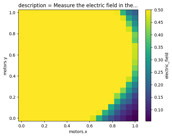
This figure exhibits some saturation: most of the measured values are fixed at \(0.5\). Let us have a look at the required configurations, using to_pseudo_data_tree(), which converts an iteration tree in a more readable format.

See also

This user guide section presents pseudo data trees more extensively.

import pprint
pprint.pprint(configs.to_pseudo_data_tree())

{'description': 'Measure the electric field in the region 0 <= X, Y <= 1.',
 'motors': {'x': LinearRange(start=0,
                             end=1,
                             default_value=_NoDefault(),
                             steps=20),
            'y': LinearRange(start=0,
                             end=1,
                             default_value=_NoDefault(),
                             steps=20)},
 'oscilloscope': {'amplitude': 1}}

The amplitude of the oscilloscope is configured to 1, and it does not have an offset, so this means that the maximum value it can measure is 0.5. This explains why we obtained saturated measurements. Let us vary the amplitude of the oscilloscope in order to find a suitable value. Here, we use replace_node() to replace the type of a node in the iteration tree. This allows us to change the fixed amplitude value of the oscilloscope with a geometrically distributed sequence.

configs = (configs
    .replace_node(["oscilloscope", "amplitude"], GeometricRange, start=1, end=10000, steps=3)
)
coords, dims_name, dims_shape = iteration_tree_to_xarray_parameters(configs)
results = xr.Dataset(
    data_vars=dict(
        electric_field=(dims_name, np.full(dims_shape, np.nan)),
    ),
    coords=coords
)

for config in configs:
    flat_config = {
        coord: v for coord, v in flatten_datatree(config).items() if coord in dims_name
    }
    factory.configure_experiment(config)
    results.electric_field.loc[flat_config] = oscilloscope.get_measurement()

results

<xarray.Dataset> Size: 10kB
Dimensions:                 (motors.x: 20, motors.y: 20,
                             oscilloscope.amplitude: 3)
Coordinates:
    description             <U56 224B 'Measure the electric field in the regi...
  * motors.x                (motors.x) float64 160B 0.0 0.05263 ... 0.9474 1.0
  * motors.y                (motors.y) float64 160B 0.0 0.05263 ... 0.9474 1.0
  * oscilloscope.amplitude  (oscilloscope.amplitude) float64 24B 1.0 100.0 1e+04
Data variables:
    electric_field          (motors.x, motors.y, oscilloscope.amplitude) float64 10kB ...

xarray.Dataset

• Dimensions:
  • motors.x: 20
  • motors.y: 20
  • oscilloscope.amplitude: 3
• Coordinates: (4)
  • description
    ()
    <U56
    'Measure the electric field in t...

    array('Measure the electric field in the region 0 <= X, Y <= 1.',
          dtype='<U56')

  • motors.x
    (motors.x)
    float64
    0.0 0.05263 0.1053 ... 0.9474 1.0

    array([0.      , 0.052632, 0.105263, 0.157895, 0.210526, 0.263158, 0.315789,
           0.368421, 0.421053, 0.473684, 0.526316, 0.578947, 0.631579, 0.684211,
           0.736842, 0.789474, 0.842105, 0.894737, 0.947368, 1.      ])

  • motors.y
    (motors.y)
    float64
    0.0 0.05263 0.1053 ... 0.9474 1.0

    array([0.      , 0.052632, 0.105263, 0.157895, 0.210526, 0.263158, 0.315789,
           0.368421, 0.421053, 0.473684, 0.526316, 0.578947, 0.631579, 0.684211,
           0.736842, 0.789474, 0.842105, 0.894737, 0.947368, 1.      ])

  • oscilloscope.amplitude
    (oscilloscope.amplitude)
    float64
    1.0 100.0 1e+04

    array([1.e+00, 1.e+02, 1.e+04])

• Data variables: (1)
  • electric_field
    (motors.x, motors.y, oscilloscope.amplitude)
    float64
    0.5 1.879 1.938 ... 0.1758 0.1797

    array([[[ 0.5       ,  1.87890625,  1.9375    ],
            [ 0.5       ,  3.2578125 ,  2.83984375],
            [ 0.5       ,  5.4296875 ,  5.4609375 ],
            ...,
            [ 0.5       ,  1.3046875 ,  1.44140625],
            [ 0.5       ,  0.93359375,  0.9296875 ],
            [ 0.5       ,  0.59375   ,  0.59765625]],
    
           [[ 0.5       ,  2.3359375 ,  2.55078125],
            [ 0.5       ,  4.25390625,  4.16796875],
            [ 0.5       ,  7.79296875,  7.66796875],
            ...,
            [ 0.5       ,  2.03515625,  2.3515625 ],
            [ 0.5       ,  1.3203125 ,  1.23046875],
            [ 0.5       ,  0.8984375 ,  0.89453125]],
    
           [[ 0.5       ,  2.953125  ,  3.2421875 ],
            [ 0.5       ,  4.79296875,  5.359375  ],
            [ 0.5       , 10.78515625, 10.109375  ],
            ...,
    ...
            ...,
            [ 0.5       ,  0.60546875,  0.61328125],
            [ 0.47265625,  0.484375  ,  0.46484375],
            [ 0.38671875,  0.33203125,  0.34375   ]],
    
           [[ 0.06640625,  0.0703125 ,  0.06640625],
            [ 0.09375   ,  0.09375   ,  0.1015625 ],
            [ 0.125     ,  0.12109375,  0.109375  ],
            ...,
            [ 0.39453125,  0.44921875,  0.4296875 ],
            [ 0.328125  ,  0.328125  ,  0.3203125 ],
            [ 0.24609375,  0.2578125 ,  0.2734375 ]],
    
           [[ 0.05078125,  0.0546875 ,  0.05859375],
            [ 0.06640625,  0.0703125 ,  0.0703125 ],
            [ 0.0859375 ,  0.08203125,  0.09375   ],
            ...,
            [ 0.28515625,  0.2734375 ,  0.30078125],
            [ 0.2421875 ,  0.2578125 ,  0.24609375],
            [ 0.19921875,  0.17578125,  0.1796875 ]]], shape=(20, 20, 3))

• Indexes: (3)
  • motors.x
    PandasIndex

    PandasIndex(Index([                0.0, 0.05263157894736842, 0.10526315789473684,
           0.15789473684210525, 0.21052631578947367,  0.2631578947368421,
            0.3157894736842105,  0.3684210526315789, 0.42105263157894735,
           0.47368421052631576,  0.5263157894736842,  0.5789473684210527,
             0.631578947368421,  0.6842105263157895,  0.7368421052631579,
            0.7894736842105263,  0.8421052631578947,  0.8947368421052632,
            0.9473684210526315,                 1.0],
          dtype='float64', name='motors.x'))

  • motors.y
    PandasIndex

    PandasIndex(Index([                0.0, 0.05263157894736842, 0.10526315789473684,
           0.15789473684210525, 0.21052631578947367,  0.2631578947368421,
            0.3157894736842105,  0.3684210526315789, 0.42105263157894735,
           0.47368421052631576,  0.5263157894736842,  0.5789473684210527,
             0.631578947368421,  0.6842105263157895,  0.7368421052631579,
            0.7894736842105263,  0.8421052631578947,  0.8947368421052632,
            0.9473684210526315,                 1.0],
          dtype='float64', name='motors.y'))

  • oscilloscope.amplitude
    PandasIndex

    PandasIndex(Index([1.0, 100.00000000000004, 10000.00000000001], dtype='float64', name='oscilloscope.amplitude'))

• Attributes: (0)

The resulting data can finally be plotted to check what has just been acquired:

Show code cell source

Hide code cell source

# Prepare an image grid
fig = plt.figure(figsize=(18, 7))
grid = ImageGrid(
    fig,
    111,
    (1, len(results["oscilloscope.amplitude"])),
    axes_pad=0.2,
    cbar_location="bottom",
    cbar_mode="each",
    cbar_pad=None,
    aspect=False,
    cbar_size="3%",
)

for (lab, data), ax, cax in zip(
    results.electric_field.groupby("oscilloscope.amplitude"), grid, grid.cbar_axes
):
    contours = ax.contour(data.squeeze(), norm=LogNorm(), colors="w")
    ax.clabel(contours, inline=1, fontsize=10)
    im = ax.imshow(data.squeeze(), interpolation="nearest", norm=LogNorm())
    cax.colorbar(im)
    ax.set_xticks([])
    ax.set_yticks([])
    ax.set_title(f"Amplitude {data['oscilloscope.amplitude'].item():.0f}")

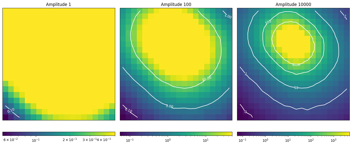
Using these measurements, the experimenter can now properly configure the amplitude of his oscilloscope, in order to measure the phenomenon of interest.

Conclusion and getting further

This example illustrates how Phileas work, and how you can prepare a simple experiment with it. Notably, it splits an experiment in three parts:

• the bench configuration file describes the instruments that are available on an experimental setup, and is not portable;

• the experiment configuration file describes what an experiment does, and is usually what the experimenter works with;

• the acquisition script handles everything else, and notably the measurements and the storage of their results.

The experiment configuration file and the acquisition script are meant to be portable. This architecture reduces the efforts required to replicate an experiment and share it with others.

Now that you have seen at a glance how to use Phileas, you can dive into more advanced examples.

You can go to the user guide to have detailed information about specific features of Phileas.